📃 This article is part of a series on Identifying Electoral Fraud Using Trend Analysis.
The simplest (yet possibly the most important) trends to start with were covered in our previous articles:
The articles mentioned above will make the following article easier to comprehend.
Historical County General Election Trends
We will first look at the historical county General Election trends to identify potential issues, and then augment the analysis with “registration” data to derive a formula for calculating excess votes, in the next article.
This analysis is fairly simple and expands on the The Fall of the Bellwether Counties concepts; to turn the historical election results for any county, into a highly accurate predictor of election outcomes.
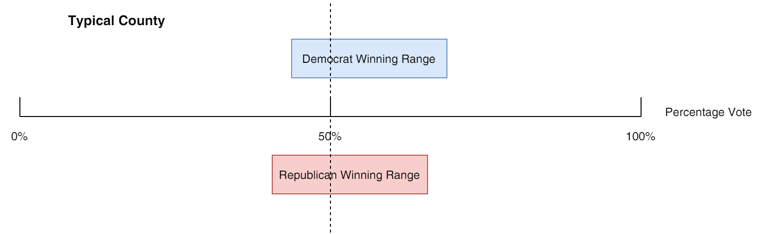
If we look more closely at what makes a “bellwether county” special, it is simply the fact that it consistently votes for the winning candidate at every election. The key is that it will vote for either party depending on the merits of each election. This means that after several elections we can derive two ranges of “winning percentages”. One for each party.
The results for a bellwether county (in this case Warren County, IL) will look like this:
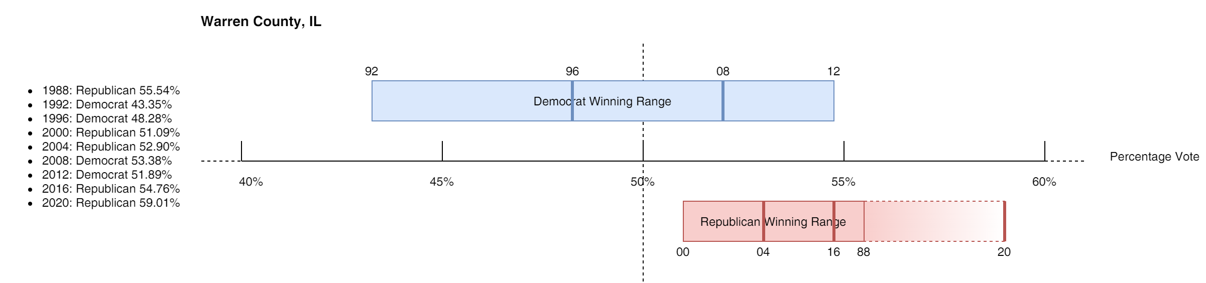
The numbers surrounding the rectangles, represent the year of the election.
The X-Axis represents that “percentage vote” for the winning party at each election.
The results for each election are shown on the left hand side of the image.
Although it’s rarer, when a county has a strong 3rd party presence, it’s possible for a party to win that county with less than 50% of the votes. (As is the case for Warren County, IL, in 1992 and 1996).
Here is an animated example showing how the ranges are updated after each election:
💡 TIP:
A picture of the 10 best bellwether’s “winning ranges” can be found here.
If we were to take this concept to the extremes we would obtain the following scenarios. (Note, the size of the ranges are exaggerated to illustrate a point):
-
A county that only voted Democrat:
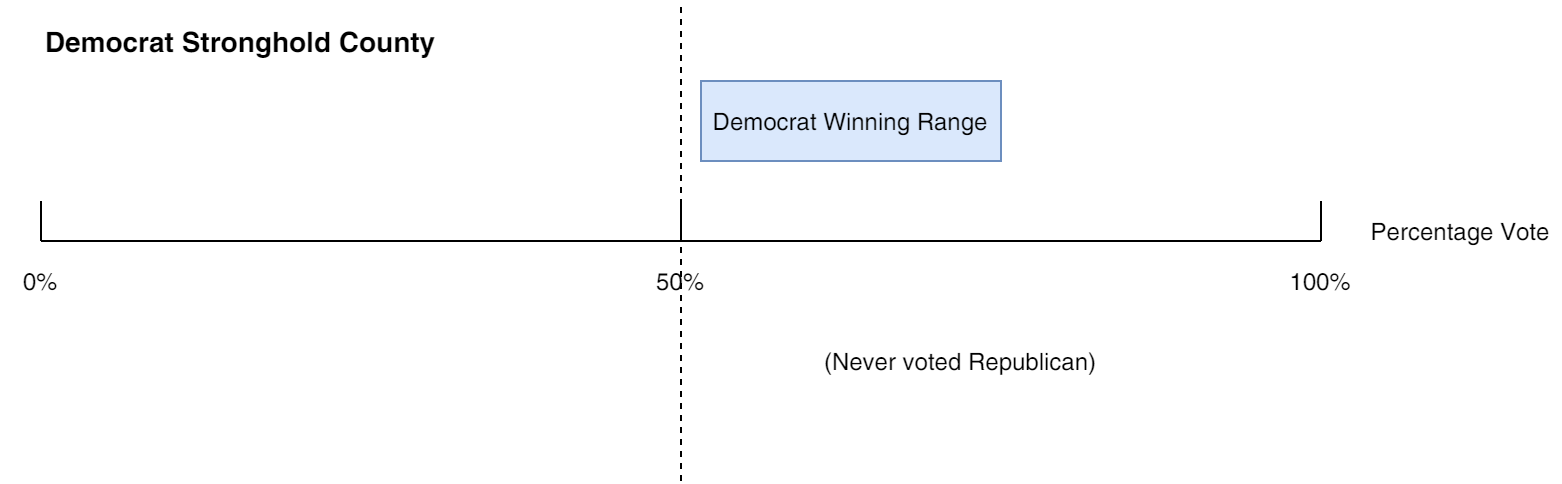
-
A county that only voted Republican:
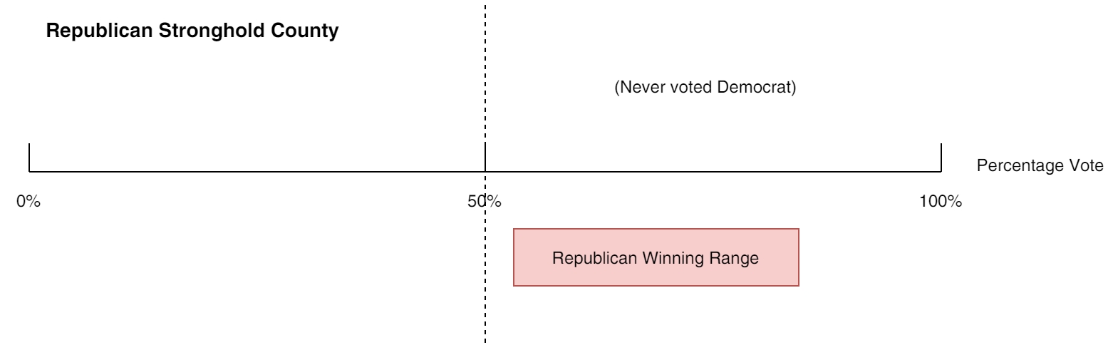
Needless to say that there are a multitude of different permutations, one of which could look like this:
💡 TIP:
This “Winning Range” is an important concept that gives us a lot of valuable information.
For example, if a county always votes Republican, it’s typical to see it vote less for the Republican candidate when a Democrat candidate wins the general election. And vice-versa.
So even though not all counties are technically “bellwether” counties, by carefully looking at their winning ranges and understanding where an election result is located within that range, we can determine if the outcome of an election makes sense or not.
In order to facilitate the analysis and compare counties with one another we will distill all this information into a single number. This number tells us where in the range of previous results did this specific election fall — did the party win a county by an average margin, a lower-than-average margin, or did they set a new winning margin record, and by how much? We’ll call it the “Location”. (The choice of this name will become clearer shortly.)
If a party wins a county by a margin that ends up in the middle of the range, the “Location” value will be close to 50%. If they only win by a small margin, that is closer to the “low” end of the range, the “Location” value will be closer to 0%. If the winning margin is lower than the “low” end of the range (i.e. a new “low” end record is set), the “Location” value will be negative. If they win with a large margin, the “Location” value will be closer to 100% or even greater than 100% if they set a new winning record. The values above 100% are the ones we’ll be particularly interested in, as they reveal which counties set new winning records, and by how much.
The different possible values are illustrated below:
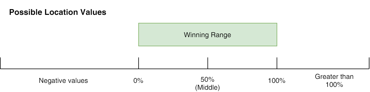
Each county’s range is updated (if required) after calculating the location value for a given election. The new range will then be used to calculate the location value at the next election.
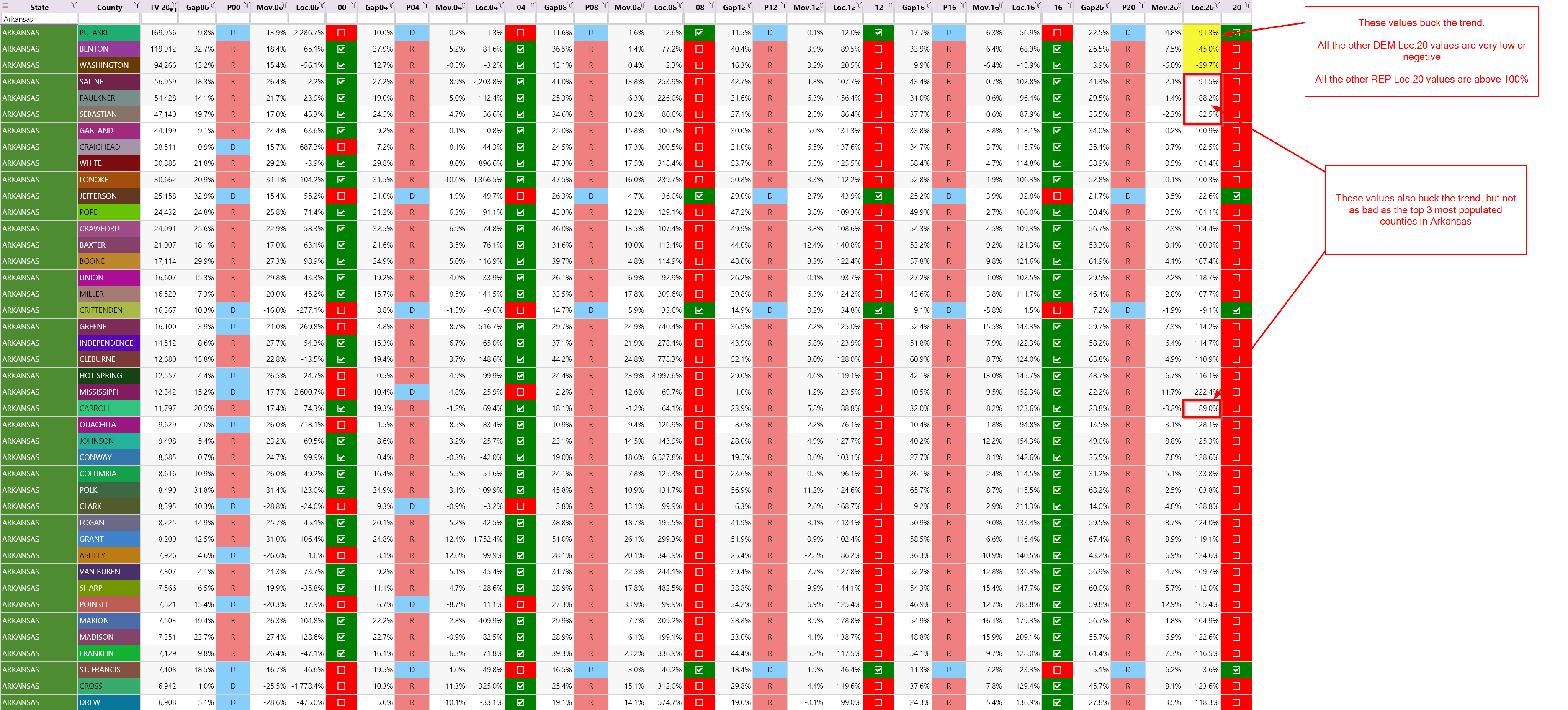
Case Study: Arkansas
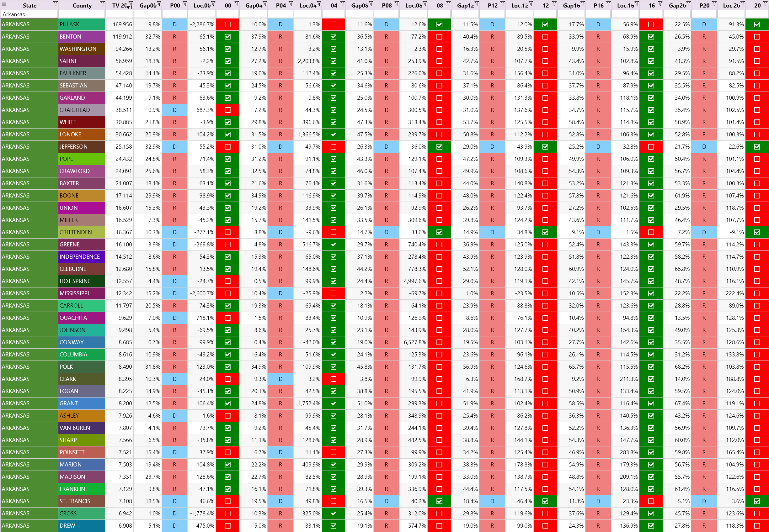
Let’s now look at the results for all the counties in Arkansas for all the elections since 2000. Arkansas is one of the cleanest states in the 2020 election, so it will give us a “baseline” against which to measure other states against. (It isn’t perfect, as we will soon see, but it is close.)
Concentrate on the Loc.20 column (the “Location” value for 2020 election), and pay attention to the trends.
In the following tables, you’ll see these columns. Here’s what they mean:
| TV20 | Total Votes in 2020 |
| Gap | Is the gap between the Winning Party Percentage - Loosing Party Percentage. This is always positive and is always relative to the winning party it is associated with, shown in column “P”. |
| P | Winning party (either “R” or “D” for “Republican” or “Democrat”) |
| Mov | Movement (or change) in winning percentage from previous election. i.e. Current Gap - Previous Gap |
| Loc | Location of the current winning percentage (as we explained above) |
| 04, 08, 12, … | True or False. Indicates whether the winning party in that county was also the winning party for the overall election. Did the county vote for the winner? |
The counties are sorted from largest to smallest total votes (i.e. the most populated counties are at the top).
As you look at the data below, think critically, and ask yourself these questions:
- What do you notice about the Republican counties Loc.20 values?
- What do you notice about the Democrat counties Loc.20 values?
- Are there any counties that are bucking the trend? Which ones?
Try and answer these questions for yourself before looking at the answers (which are given in the “Observations” section below).
(Two screenshots were needed to capture all the counties. Click an image to enlarge it.)
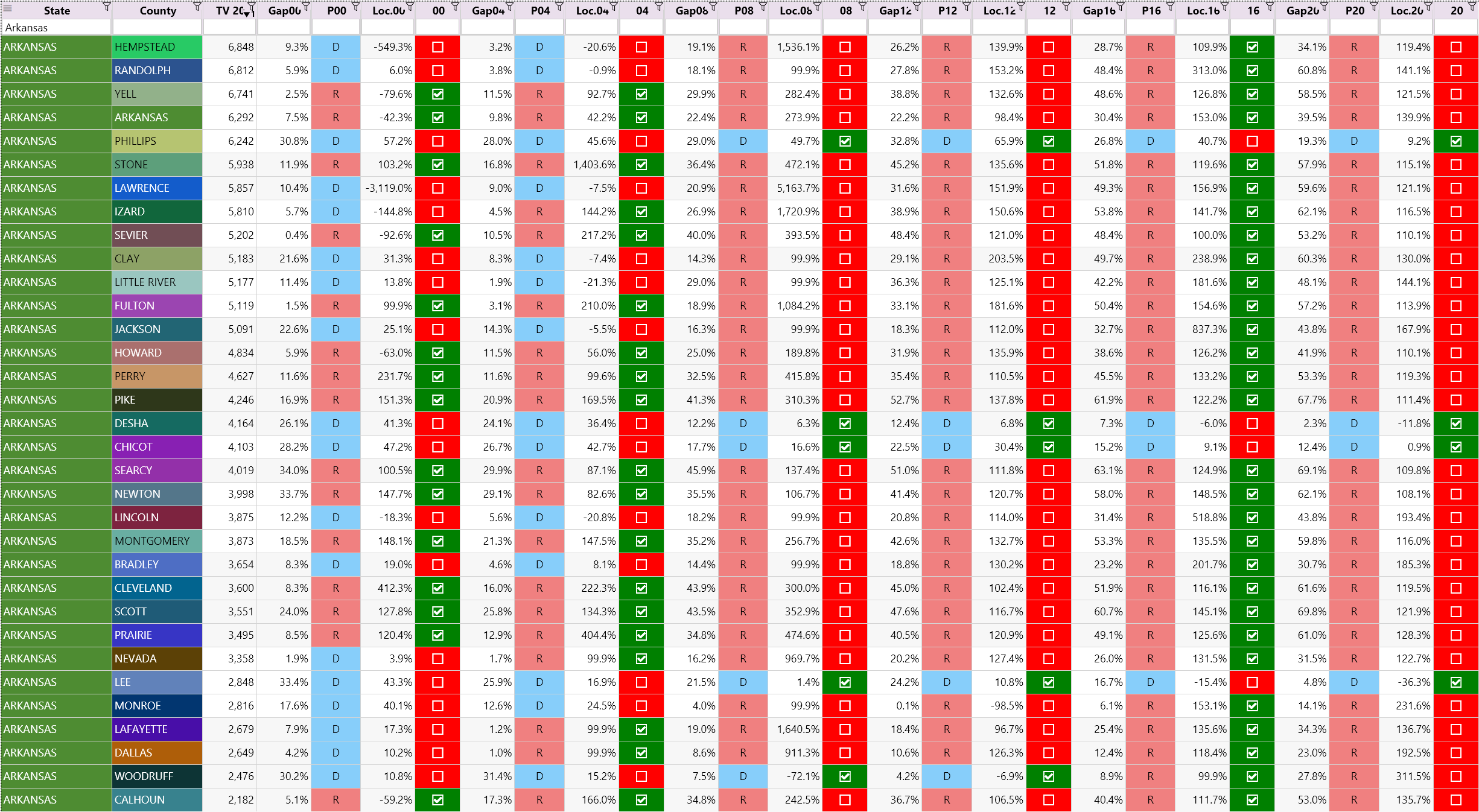
Observations
- Most counties voted very strongly Republican, setting a new record margin, with a Loc.20 value over 100%.
- The 3 most populated counties buck the trend.
- The Loc.20 value for Pulaski is much higher than all the other Democrat county values.
- The Loc.20 value for Benton and Washington is much lower than all the other Republican county values.
- All the other counties strongly voted Republican in 2020 with a Loc.20 value exceeding 100% across the board. This means they set individual new record highs for the Republican winning range.
Here are the same images as before, but this time with a new “Movement” column. This represents the change in “Gap” value from the previous election to the current election. This column helps quantify the shift in sentiment between elections and is simply added as a reference to help people understand the usefulness of the “Location” column to quickly identify anomalies.

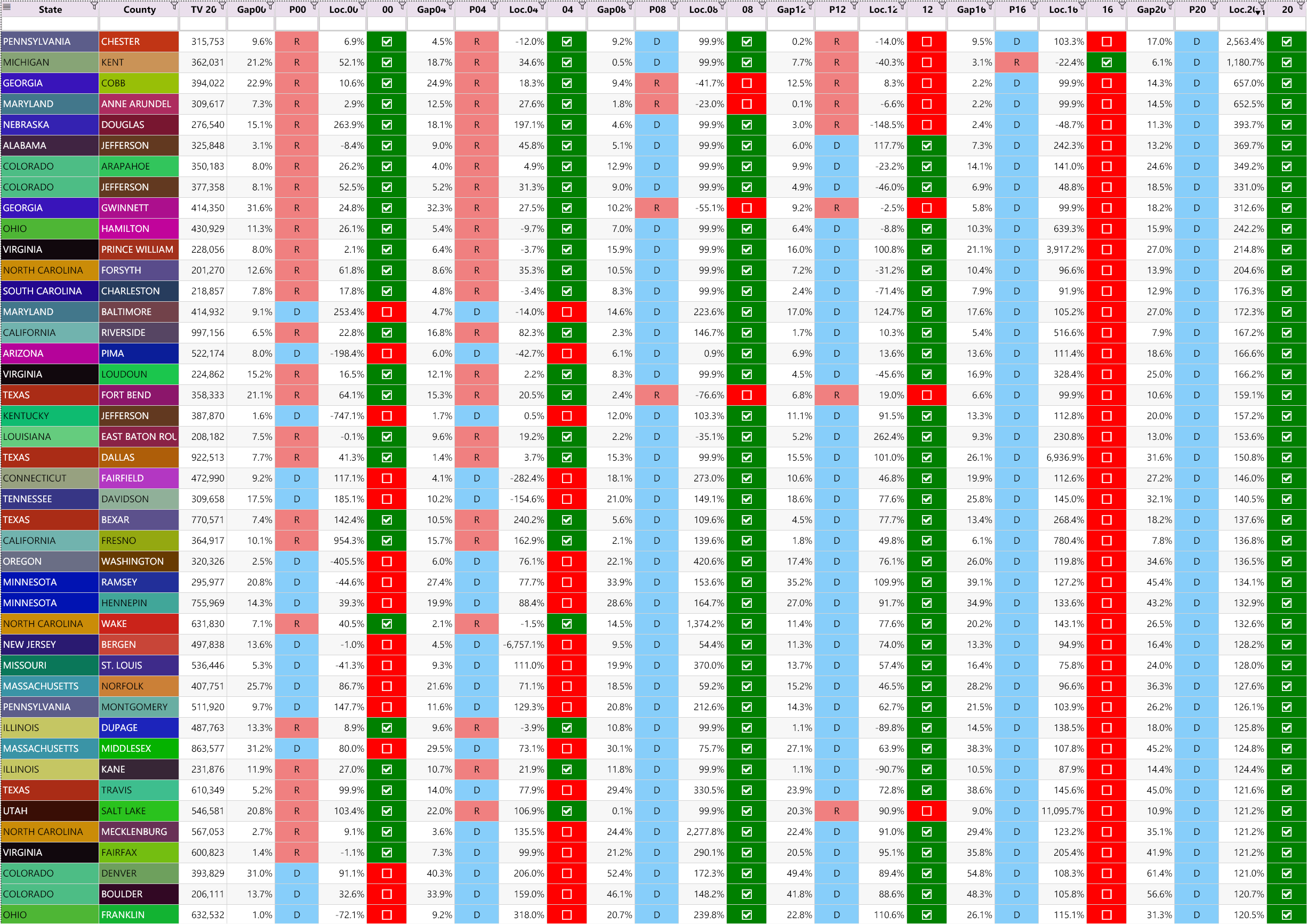
Case Study: Counties with Over 200K Votes
We recommend reading The Battle of the Largest Counties article first, if you haven’t already. It will provide the necessary background to assist you in finding meaningful trends.
So now let’s look at the counties with a total vote greater than 200K, sorted by descending order of their Loc.20 value (from highest to lowest). These are the large counties that set huge new winning margin records in the 2020 election.
Take some time to look at the data. Try and identify some trends on your own, before reading the observations.
So what did you notice?
Here is what we observed:
-
There is no trickery in the tables above. There really are no Republican counties with over 200K votes that have a Loc.20 value over 100%. (In other words, no Republican county with over 200K votes, increased their percentage lead from 2016 to 2020.)
-
The fact that all these counties are uniformly Democrat is completely abnormal (especially when considering that the Republican party increased their votes by a record 10+ million over the previous election).
-
Why did all the larger Democrat counties perform so well at the 2020 election and all the smaller Democrat counties perform so poorly? (From a trend analysis point of view, this is one of the basic yet most compelling “tell-tale” signs that something does not add up.)
-
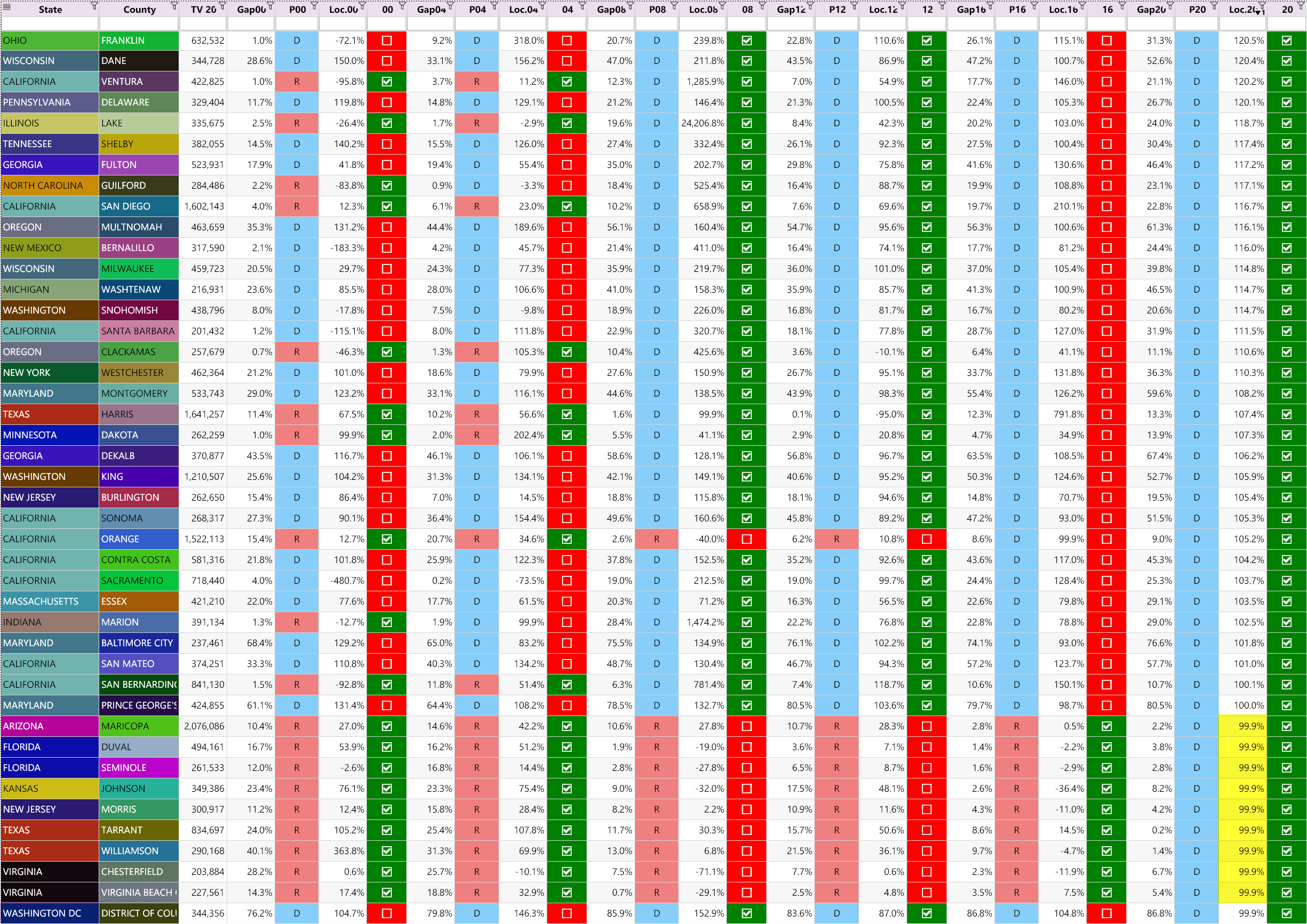
Counties with a Loc.20 value over 120% warrant further investigation. Expanding a range by 20% is suspicious, especially for counties with over 200K votes. (It just so happens that the first image only contains counties with a Loc.20 value greater than 120% in 2020.)
-
In the second image, we highlighted counties that voted Democrat for the first time in 2020. Notice their total votes in 2020 (the TV20 column). Do you notice a trend?
-
Notice how many counties used to vote Republican in 2000, and have gradually turned blue by 2020. (Is this part of a master plan to gradually turn all the largest counties blue?)
-
Do all these trends make sense to you?
Here is the list of all the most populated counties sorted by their total votes in 2020. You will notice the Republican counties are sparse, and their LOC.20 value is always less than 100%. We find this abnormal considering Trump had an extra 10+ million people vote for him in 2020. The highest of any incumbent President, ever.
What this means is that no Republican counties with over 200K votes increased their percentage lead from 2016 to 2020. It does not mean the total Republican votes did not increase. All of them did! It just means the total Democrat votes, in each of the large counties, increased more than the Republican votes (even within Republican strongholds!).
What makes this all the more confounding is that this trend only applies to populated counties. In smaller Democrat stronghold counties, with stable population growth, we observe large swings towards the Republican party.
Something does not add up.
We will leave you with a quote from Seth Keshel to ponder…
How is California turning every state in the west more blue, blue, or purple, while doubling it’s own blue votes since 2000?
Let the one with wisdom understand.
Summary
Hopefully you’ve learnt a few new tools for analyzing election results by comparing the results with earlier years, and calculating a number that represents how the result compared to previous years.
This “Historical County Range Analysis” can provide compelling information about the historical trend for an individual county, as well as a state wide trend for how the counties voted for a particular party.
You should have already noticed a few intriguing statistics that deserve a closer look. In the following article we’ll dig deeper and incorporate voter registration data, which will allow us to derive a formula for estimating excess votes.
Other Articles In This Series
| Overview | Diving deeper into the unusual trends and statistics discovered in the 2020 election. |
| Part 1 | A look at the surprising failure of the bellwether counties in 2020, and what that tells us about the Presidential election outcome. |
| Part 2 | The data shows the Democrats are winning less and less counties at each election, but are winning more and more of the largest counties. How is this possible? |
| Part 3 | Voter turnout rates shot up dramatically in many states in 2020. We look at the voting rates since 2000 to find out which states set a new record. |
| Part 4 |
When Winning Margins Go “Off the Charts”
Learn how to "normalize" a county's winning margin to identify abnormalities. What does this reveal about the 2020 election?
|
| Part 5 | Learn how to use the party registration numbers for each county to predict the election results for a state and assess the likely validity of the results. This is a guide on the method Seth Keshel uses for his predictions and county heat maps, allowing you to dig into the trends of your own county and uncover anomalies. |
| Part 6 | We build on some of the previous techniques to scan 3,111 American counties, identifying those whose shift in vote totals moves unexpectedly against the shift in party registrations. |
| Part 7 | We compare the Democrat vote totals with previous elections which reveal some very large increases in unlikely places. |
| Part 8 | We compare key parameters in the 2020 results against the previous five elections using the z-score, and find hundreds of counties breaking statistical norms. |
| Part 9 | Interesting statistical findings on how the Presidential race results compared to the other races in the same election. |
| Part 10 |
Voter Roll Analysis
Coming soon.
|
| Part 11 |
The Art of the Steal
Coming soon.
|
Follow us on Telegram to be notified when we release the remaining articles.
Visitor Comments
Did you find this article helpful? Did you dig in and review the data for your county or state? What did you find? Let us know in the comments below.